Scaling Analysis and Modeling
There are four kinds of lies: Lies, Damn Lies, Statistics, and Visualizations
—Nathaniel S. Borenstein
In this chapter the question of how calibration time \(T\) scale with the number of available processing units (PUs) \(n\) will be examined. It is possible to perform two types of scaling analyses, one where the size of the problem stays fixed and one where it varies with the number of PUs. As customary, I will refer to them as weak scaling and strong scaling respectively. What do I mean by size of the problem in the context of derivative-free optimization? One obvious answer is the number of function evaluations, or budget, in the parlance of the Nevergrad library; but this number is a random variable when we resample after failing computations. Nonetheless, the budget is the infimum for the actual number of function evaluations and optimizer.tell calls, which is the amount of information collected by the optimizer. Therefore, the budget is a good definition for the size of the problem after all, as long as one keeps in mind that he is dealing with a stochastic process. Indeed, each particular realization will not depend in a deterministic way on parameters such as the budget. However, changing the budget will change the distribution, and the mean value of calibration time in a deterministic way.
For evolutionary algorithms the budget is given by the number of individuals \(p\) times the number of generations \(g\). For these algorithms, as more thoroughly explained in previous chapters, changing the population size can have large effects on the result and execution time of optimization. Indeed, the population size determines, on the one hand, the probability of escaping from a local minimum and, on the other, the degree to which optimization can be executed in parallel. The latter statement, for which we have developed an intuition based on the arguments in the previous chapters, will be given a quantitative form later on in this one. For the previous reasons, in the following I will consider \(p\) as the size of the problem, and the number of generations \(g\) fixed.
import scrapbook as sb
import numpy as np
import seaborn as sns
import matplotlib.pyplot as plt
import statsmodels.formula.api as smf
from datetime import timedelta
from mhpc_project.utils import get_scaling_data
from scipy.optimize import curve_fit

plt.rcParams.update({'figure.figsize':(16,9), 'figure.dpi':100})
Scaling and Efficiency
Strong Scaling
In this analysis, the calibration notebook has been executed several times with increasing \(n\) while keeping \(p\) fixed. This is done using Papermill, which allows parametrizing and executing Jupyter notebooks in an automated way. Later, using the Scrapbook library, it is possible to recover the objects defined during the execution (which are serialized and saved within the notebook) and the metadata saved by Papermill, such as the notebook execution time.
The Scrapbook library offers the convenience function read_notebooks that takes the path to a directory and returns a scrapbook. This object has an iterator interface that yields the notebooks within that directory, and that can be used to collect the data from an ensemble of notebooks.
strong_scaling_book = sb.read_notebooks('../runs/strong_scaling')
We can retrieve the data relevant to scaling using the get_scaling_data function from mhpc_project.utils. This function takes a scrapbook and for each of its notebooks checks that every code cell has been successfully executed and, if so, it stores its data in a Pandas dataframe.
strong_scaling_data =  get_scaling_data(strong_scaling_book)
strong_scaling_data.head()
| name | num_cpus | popsize | num_generations | ratio | duration | num_samples | samples_duration | num_good_samples | good_samples_duration | efficiency | speedup | |
|---|---|---|---|---|---|---|---|---|---|---|---|---|
| 0 | testbed-NGO-4096-1024-40d | 1024 | 512 | 8 | 0.5 | 1610.952014 | 4932 | 545846.852303 | 4096 | 421527.591743 | 0.255531 | 15.183880 |
| 1 | testbed-NGO-4096-1024-7oK | 1024 | 512 | 8 | 0.5 | 1885.252965 | 4953 | 551817.418133 | 4097 | 425539.367783 | 0.220430 | 12.974652 |
| 2 | testbed-NGO-4096-1024-BkB | 1024 | 512 | 8 | 0.5 | 1630.464289 | 5002 | 556402.759809 | 4096 | 422624.253288 | 0.253130 | 15.002170 |
| 3 | testbed-NGO-4096-1024-CoT | 1024 | 512 | 8 | 0.5 | 1636.694933 | 4871 | 537770.736557 | 4096 | 423323.413666 | 0.252583 | 14.945059 |
| 4 | testbed-NGO-4096-1024-KpN | 1024 | 512 | 8 | 0.5 | 2286.894785 | 5020 | 556299.929107 | 4097 | 420288.756369 | 0.179474 | 10.695945 |
As noted above, the calibration time is a random variable and, as shown by the entries in the previous dataframe, it can vary widely from one realization to another, although with the same parameters. However, we will be mainly concerned with its mean value \(T\), and, if not explicitly stated otherwise, I will refer to mean values when talking about execution times (the same goes for its derived quantities).
The speedup \(S\) is usually defined as
However, since we don’t have a serial execution as a reference, the following definition will be used
where in our case \(n_0 = 32\). In case of perfect (linear) strong scaling, \(T\) is inversely proportional to \(n\), and we have
It is possible to improve this simple model of the computation by including the effect of the population size. If the objective never fails, each PU exceeding the population size will idle. Hence, we can have perfect scaling only up to \(n = p\)
ax = sns.lineplot(data=strong_scaling_data, x='num_cpus', y='speedup',
             err_style='bars', marker='o', label='data')
sns.lineplot(x=strong_scaling_data['num_cpus'], y=strong_scaling_data[['num_cpus', 'popsize']].min(axis=1) / strong_scaling_data['num_cpus'].min(),
             label='reference', ax=ax)
ax.set_title('Strong Scaling (popsize = 512)')
plt.show()
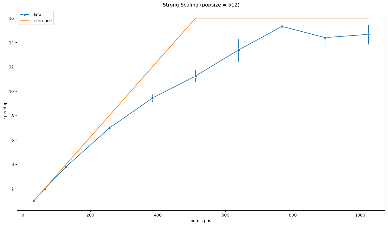
As can be evinced from the plot above, the simple model described by the equation {eq}`eq:max_speedup} seems to be very effective. It is interesting to note that the execution appears to reach values near the theoretical maximum speedup, but with \(n\) sensibly larger than \(p\). One possible interpretation is that, as we know, the effective population size is larger than \(p\) due to objective function failures. However, in that case the speedup should be also larger than \(p / n_0\). In principle, knowing the statistics of the objective execution times and failures, it should be possible to model more accurately the calibration speedup. However, I will use a simpler approach based on data.
Efficiency
Another interesting quantity is the efficiency, defined as the fraction of time spent by a PU computing the values of the objective actually told to the optimizer
By definition, the remaining part of time is spent idle, computing NaNs or unused values.
sns.lineplot(data=strong_scaling_data, x='num_cpus', y='efficiency', err_style='bars')
plt.show()
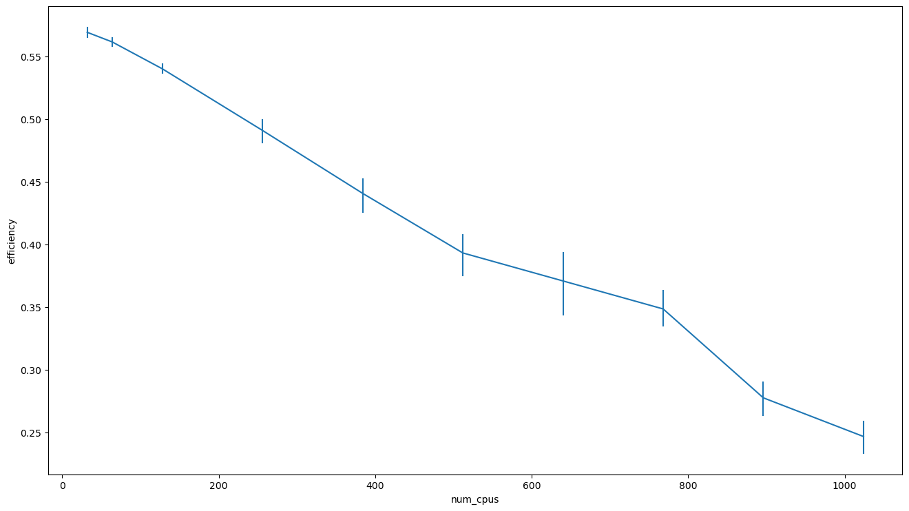
It is worth noting that while we can get a speedup by using more PUs, the efficiency will drop.
Weak Scaling
In weak scaling analysis, the calibration notebook has been executed several times with increasing \(p\) and \(n\), while keeping the ration \(p / n\) fixed. Note that from strong scaling analysis we know that larger \(p / n\) values correspond to smaller errors.
In case of weak scaling, the speedup is not a meaningful metric, since the size of the problem changes. Instead, we are interested in the execution time \(T\), and perfect scaling happens when \(T\) is constant.
weak_scaling_book = sb.read_notebooks('../runs/weak_scaling')
weak_scaling_data = get_scaling_data(weak_scaling_book)
ax = sns.barplot(data=weak_scaling_data, x='num_cpus', y='duration',
             label='data', capsize=0.2, color="#1f77b4")
ax.yaxis.set_major_formatter(lambda value, position: timedelta(seconds=value))
ax.set_title('Weak Scaling (num_cpus = popsize)')
plt.show()
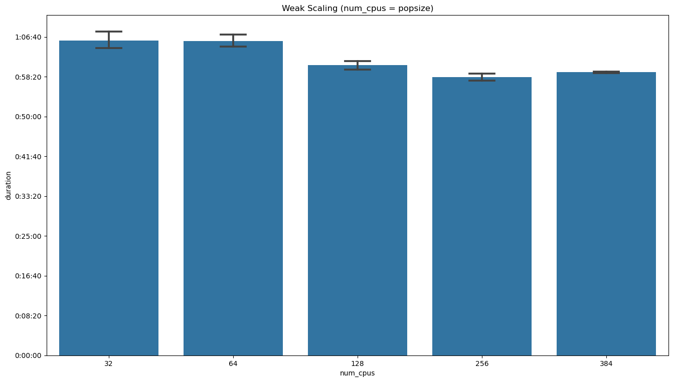
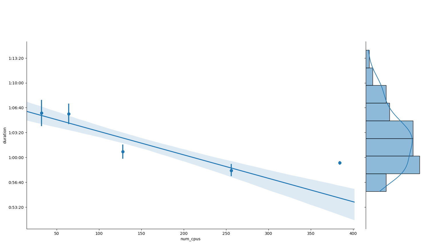
Visual inspection suggests that the hypothesis of perfect weak scaling is compatible with the data within the errors. The same thing can be shown by means of linear regression in the plot and summary below.
grid = sns.JointGrid(data=weak_scaling_data, x='num_cpus', y='duration')
grid.fig.set_figwidth(16)
grid.fig.set_figheight(9)
grid.plot_joint(sns.regplot, x_estimator=np.mean, truncate=False)
grid.ax_marg_x.set_axis_off()
sns.histplot(data=weak_scaling_data, y='duration', kde=True, ax=grid.ax_marg_y)
grid.ax_joint.yaxis.set_major_formatter(lambda value, position: timedelta(seconds=value))
plt.show()

smf.ols(formula='duration ~ 1 + num_cpus', data=weak_scaling_data).fit().summary()
| Dep. Variable: | duration | R-squared: | 0.531 |
|---|---|---|---|
| Model: | OLS | Adj. R-squared: | 0.524 |
| Method: | Least Squares | F-statistic: | 72.55 |
| Date: | Wed, 17 Feb 2021 | Prob (F-statistic): | 3.95e-12 |
| Time: | 10:57:35 | Log-Likelihood: | -432.59 |
| No. Observations: | 66 | AIC: | 869.2 |
| Df Residuals: | 64 | BIC: | 873.5 |
| Df Model: | 1 | ||
| Covariance Type: | nonrobust |
| coef | std err | t | P>|t| | [0.025 | 0.975] | |
|---|---|---|---|---|---|---|
| Intercept | 3997.5967 | 35.440 | 112.798 | 0.000 | 3926.797 | 4068.397 |
| num_cpus | -1.8878 | 0.222 | -8.518 | 0.000 | -2.331 | -1.445 |
| Omnibus: | 7.769 | Durbin-Watson: | 1.713 |
|---|---|---|---|
| Prob(Omnibus): | 0.021 | Jarque-Bera (JB): | 7.190 |
| Skew: | 0.779 | Prob(JB): | 0.0275 |
| Kurtosis: | 3.434 | Cond. No. | 267. |
Notes:
[1] Standard Errors assume that the covariance matrix of the errors is correctly specified.
Linear Scaling Model
Previous results make sense since, without further assumptions, neither perfect weak scaling imply perfect strong scaling (as would contradict our observations), nor vice-versa. Also, the way in which we measure the problem size affects weak scaling. Howeer, if the execution time is proportional to the problem size, then one form of scaling imply the other.
This fact is more evident in equations than words: the two contitions are
hence, if \(T(p, n) \propto p\), then one imply the other.
More often, a sensible requirement on the size \(p\) is just that \(T(p, n) \sim \mathcal{O}(p)\). In this sense, choosing the population size \(p\) as the problem size seems very reasonable. Indeed, it is plausible, as a first approximation, that the fraction of successful objective function calls stays constant as we change \(p\): hence, the required amount of computation goes asymptotically as \(p\).
What we can deduce from the previous analyses? From perfect weak scaling we know that \(T\) is a function of \(p / n\) alone. From strong scaling we know that the speedup for large \(n\) seems to saturate at a non-zero value, which means that \(T\) cannot have neither poles nor zeros for finite (of course, non-negative) \(p / n\). Therefore, the simplest form for \(T\) is a linear model
Let’s see if this model fits the data and what can be deduced from it.
data = strong_scaling_data
ax = sns.regplot(data=strong_scaling_data, x='ratio', y='duration', x_estimator=np.mean, truncate=False)
ax.yaxis.set_major_formatter(lambda value, position: timedelta(seconds=value))
plt.show()

fit = smf.ols(formula='duration ~ 1 + ratio',data=data).fit()
fit.summary()

| Dep. Variable: | duration | R-squared: | 0.998 |
|---|---|---|---|
| Model: | OLS | Adj. R-squared: | 0.998 |
| Method: | Least Squares | F-statistic: | 9.484e+04 |
| Date: | Wed, 17 Feb 2021 | Prob (F-statistic): | 4.06e-219 |
| Time: | 10:57:36 | Log-Likelihood: | -1116.9 |
| No. Observations: | 158 | AIC: | 2238. |
| Df Residuals: | 156 | BIC: | 2244. |
| Df Model: | 1 | ||
| Covariance Type: | nonrobust |
| coef | std err | t | P>|t| | [0.025 | 0.975] | |
|---|---|---|---|---|---|---|
| Intercept | 692.1514 | 28.355 | 24.410 | 0.000 | 636.142 | 748.161 |
| ratio | 1478.7292 | 4.802 | 307.957 | 0.000 | 1469.244 | 1488.214 |
| Omnibus: | 56.222 | Durbin-Watson: | 1.968 |
|---|---|---|---|
| Prob(Omnibus): | 0.000 | Jarque-Bera (JB): | 132.789 |
| Skew: | 1.533 | Prob(JB): | 1.46e-29 |
| Kurtosis: | 6.281 | Cond. No. | 7.43 |
Notes:
[1] Standard Errors assume that the covariance matrix of the errors is correctly specified.
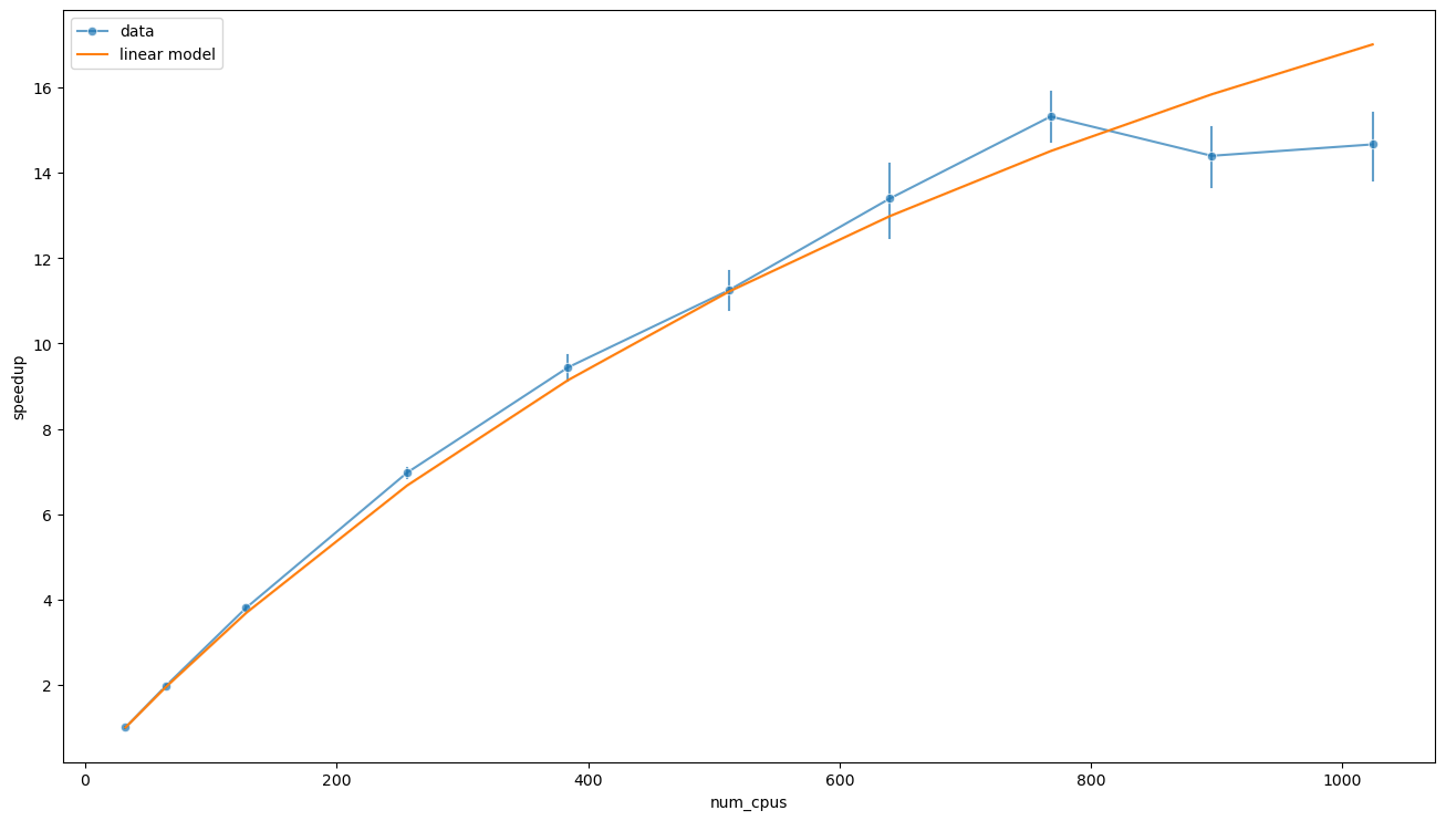
Linear regression of the optimization time \(T\) gives a strong indication that equation (2) might be the right candidate. The same functional relation can be represented also in the scaling plot.
ys=(fit.params[0] + fit.params[1] * 512 / 32) / fit.predict(data['ratio'])
sns.lineplot(data=data, x='num_cpus', y='speedup', alpha=0.7, marker='o', err_style='bars', label='data')
sns.lineplot(x=data['num_cpus'], y=ys, label='linear model')
plt.show()
We can also explicitly calculate the speedup
and compare this expression with the Amdahl’s law (corrected to use \(T(p, n_0)\) as a reference)
where \(f\) is the fraction of the program that can benefit from the speedup.
Therefore, we have that
or, equivalently, that the fraction of time that the program spend in serial code (that is not split among PUs, i.e. the internals of the optimizer) is approximately the 3%. Note that this has nothing to do with the data dependency that exists between a generation of individuals and the next, which actually limits the possibility to scale the execution on larger numbers of PUs.
We can also calculate the maximum speedup
which is sensibly higher than predicted using the simple model based on the assumption of perfect strong scaling up to \(p\).
In this case, the previous argument would suggest an effective population size of \(p_\text{eff} \approx n_0 S_\text{max} \approx 1120\) individuals. The new estimate of \(S_\text{max}\) is however too high, and the reason is that the linear model considered fails for small \(p / n\), that is large \(n\). We will address this issue later.
We can use the formula for \(T\) also to express the efficiency. Since the number of optimizer.tell calls is approximately \(p\), then, for large enough \(p\), we can approximate the sum in the definition of \(\eta\) as \(g\) times \(p\) times the mean execution time of successful computations \(\langle t_\text{s} \rangle\)
average_sample_duration = (data['good_samples_duration'] / data['num_good_samples']).mean()
predicted_efficiency = data['num_generations'] * average_sample_duration / (fit.params[1] + fit.params[0] * data['num_cpus'] / data['popsize'])
sns.lineplot(data=data, x='num_cpus', y='efficiency', alpha=0.7, marker='o', err_style='bars', label='data')
sns.lineplot(x=data['num_cpus'], y=predicted_efficiency, label='linear model')
plt.show()
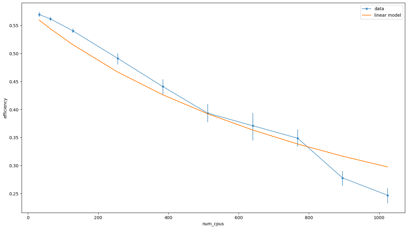
The maximum efficiency is reached for \(n \ll p\) and is equal to
data['efficiency'].max(), (data['num_generations'] * data['good_samples_duration'] / data['num_good_samples']).mean() / fit.params[1]
(0.5826281218414213, 0.5756400950552586)
The story holds up: on the one hand, \(g p T_1\) is the amount of work that can be split among workers, i.e. the average computation time times the budget. On the other, if we consider a serial execution with a large population (that is \(n = 1\) and \(p \gg 1\)), then the efficiency is the ratio between the average time spent on a successful computation and the average computation time per unit budget \(\langle t \rangle\). In both cases \(T_1 = g \langle t \rangle\). Therefore, the maximum efficiency is \(\eta_\text{max} = \frac{\langle t_\text{s} \rangle}{\langle t \rangle}\), and is characteristic of the objective function, the optimizer and the timeout.
Also, notice that there is an implicit dependency on \(g\) in \(T_1\), and hence in \(\langle t \rangle\). Indeed, as the generations pass, the optimizer explores regions the search space associated to smaller and smaller losses, and it is plausible that the objective function fails less and less. Hence, the value of \(\langle t \rangle\) calculated within a generation is expected to decrease from one generation to the next. In principle, there could be a also a dependency on \(p\), but the data for large values of \(p / n\) seems to exclude that (more on this topic in the next section).
Therefore, we can estimate \(T_1\) from the data in this other way.
t1_estimate = (data['num_generations'] * data['samples_duration'] / data['num_good_samples']).mean()

fit.params[1], t1_estimate
(1478.7292162544938, 1222.7824143247535)
Notice that \(\langle t \rangle\) can be larger than the timeout of the objective function. The reason is that there could be multiple failing computations per successful one.
Models for Large Numbers of CPUs
The previous model fails to describe the situation for large \(n\). The reason is that when \(n\) is larger than the effective population size, adding more PUs should decrease sublinearly the execution time. Indeed, if we neglect the effects due to the statistics of successful computations, \(T\) should be constant. For this reason, I considered other two models which introduce a scale \(x_0\) for \(p / n\) separating the two regimes.
The first one is a piecewise linear function
the other one is the lowest order rational function with vanishing slope at the origin and same asymptotic behaviour
We can fit the speedup using these models for the execution time. Since the speedup is defined as a ratio, it does not depend on the unit of measure of \(T\). This also means that it is not a function of both \(T_0\) and \(T_1\) but depends only on their ratio. Since the behaviour we are trying to capture is at \(p / n \to 0\), the three models are asymptotically equivalent, and the error on \(T_1\) in the fit of the linear model is small, it is convenient to consider \(T_1\) fixed to the previously calculated value.
We can now fit the piecewise model,
def speedup_from_t(t, n, params, p=512, n0=32):
    return t(np.asarray([p / n0]), *params) / t(p / n, *params)

def t_pwise(xs, t0, t1, x0):
    return np.apply_along_axis(lambda col: np.piecewise(col, [col >= x0, col < x0], [lambda x: t0 + t1 * (x - x0), t0]), 0, xs)

(t0_pwise, x0_pwise), cov = curve_fit(lambda x, t0, x0: speedup_from_t(t_pwise, x, [t0, fit.params[1], x0]),
                                      data['num_cpus'], data['speedup'],
                                      bounds=[(0.5 * fit.params[1], 0.4),(2 * fit.params[1], 0.8)])
(t0_pwise, x0_pwise), np.sqrt(np.diag(cov))
((1641.178379546566, 0.6792061302521527), array([17.60840277, 0.02223963]))
and plot the results
ax = sns.lineplot(x=data['num_cpus'], y=speedup_from_t(t_pwise, data['num_cpus'], [t0_pwise, fit.params[1], x0_pwise]), label='piecewise linear model')
sns.lineplot(data=data, x='num_cpus', y='speedup', alpha=0.7, marker='o', err_style='bars', label='data', ax=ax)
plt.show()
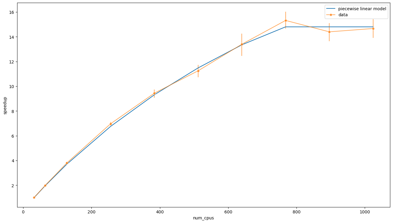
Visual inspection confirms that there is a good overlap between the data and this model. Indeed, there might even be overfitting. We can also interpret \(T_0\) and \(x_0\) and use their values to calculate the maximum speedup, which is
This value is basically the average speedup at \(n = 1024\).
The parameter \(T_0\) is the lower bound for the execution time (i.e. when the work is split among infinite PUs), and the value of \(T_0 \approx 27\text{m}\) is much more reasonable than \(T_0 \approx 14\text{m}\) found in the linear model. Indeed, in the limit \(p / n \to 0\), we can estimate this parameter
where \(\Delta T_0\) is the amount of time spent by the system starting the Dask cluster, doing plots, etc. We can calculate this number using the available data
t0_pwise - (data['num_generations'] * data['good_samples_duration'] / data['num_good_samples']).mean()
789.9625529408412
that is \(\Delta T_0 \approx 13\text{m}\).
It is also interesting to explicit the meaning of \(x_0\). In the piecewise model this parameter is the value of \(p / n\) at which the time abruptly stops scaling: this means that the number of PUs has exceded the effective population, hence
This value is also the optimal number of PUs.
We can fit in the same way the rational model
def t_rat(x, t0, t1, x0):
    return t0 + t1 * x0 * (x / x0) ** 2 / (1 + (x / x0))


(t0_rat, x0_rat), cov = curve_fit(lambda x, t0, x0: speedup_from_t(t_rat, x, [t0, fit.params[1], x0]),
                                            data['num_cpus'], data['speedup'], bounds=(0, np.inf))
(t0_rat, x0_rat), np.sqrt(np.diag(cov))
((1286.5499151493627, 0.9916561641074632), array([34.62543519, 0.18726127]))
plot the result
ax = sns.lineplot(x=data['num_cpus'], y=speedup_from_t(t_rat, data['num_cpus'], [t0_rat, fit.params[1], x0_rat]), label='rational function model')
sns.lineplot(data=data, x='num_cpus', y='speedup', alpha=0.7, marker='o', err_style='bars', label='data', ax=ax)
plt.show()
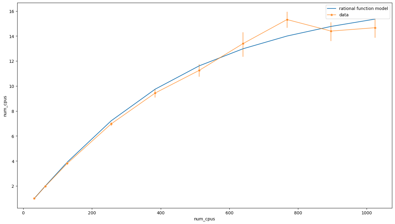
and see that the behaviour at large \(n\) is quite different. In this case we have
Also, in this case, the estimated serial time
t0_rat - (data['num_generations'] * data['good_samples_duration'] / data['num_good_samples']).mean()
435.3340885436379
is much less, \(\Delta T \approx 7\text{m}\).
All in all, the piecewise linear model seems to fit better the data, although it is a bit less realistic. Putting all together we have
where \(\langle t_\text{s} \rangle\) depend on the objective, \(\eta_\text{max}\) on the objective and the algorithm, and \(x_0\) (hence \(p_\text{eff}\)) on the objective, the algorithm and on \(g\). For optimization algorithms where there is no notion of convergence, such as random search, \(x_0\) does not depend on \(g\). For the others, the value of \(p_\text{eff}\) is expected to decrease for increasing \(g\), since, as the generations pass, the objective should fail less and less. If one considers the change of \(x_0\) due to \(g\) negligible, the previous formula allows estimating the scaling of calibration for a fixed combination of objective and algorithm using only two points, and only one point if \(\Delta T_0\) is known.
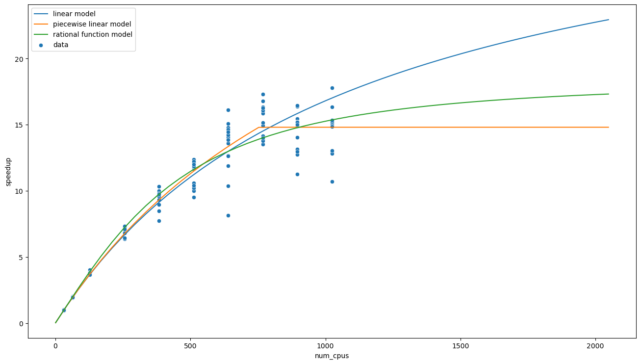
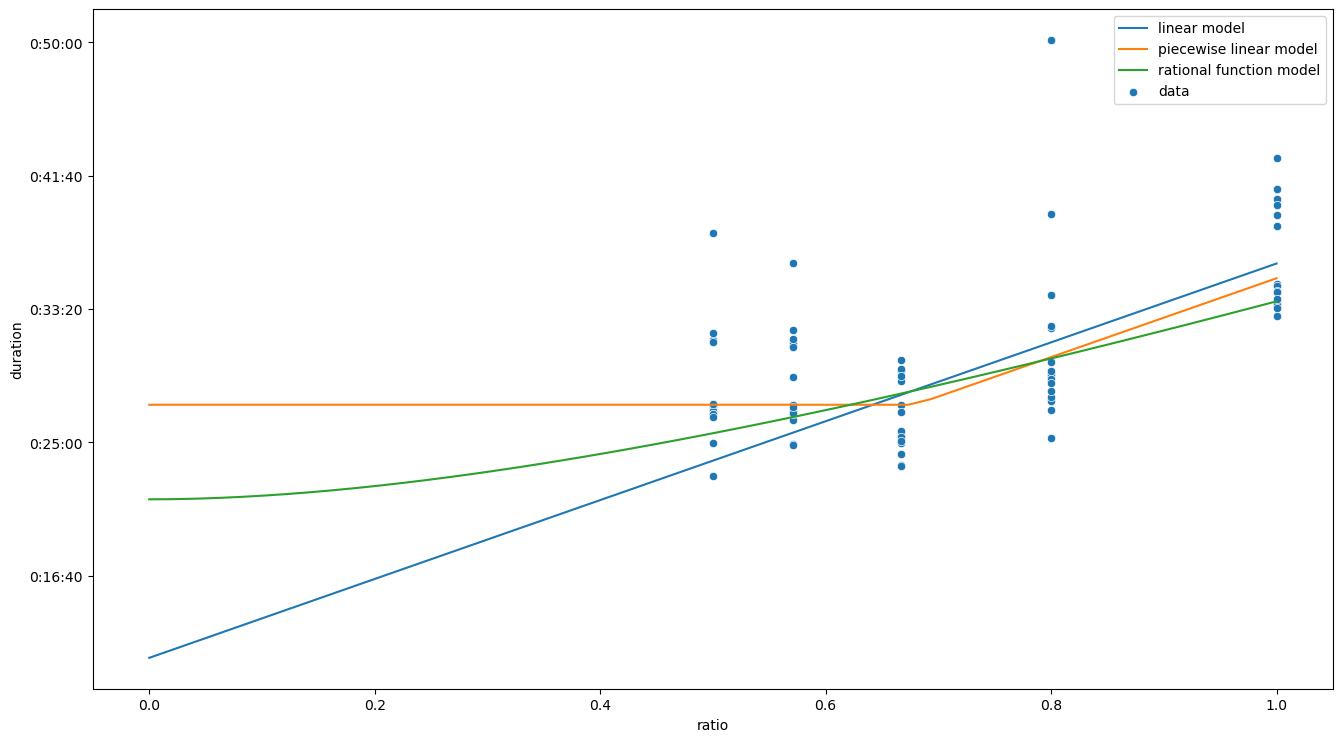
Finally, it is instructive to take a look at the different models for execution times near \(p / n \to 0\), or equivalently to the speedups at \(n \gg p\).
xs = np.linspace(0, 1)
ax = sns.scatterplot(data=data[data['ratio'] <= 1.0], x='ratio', y='duration', estimator=np.mean, label='data')
sns.lineplot(x=xs, y=fit.params[0] + fit.params[1] * xs, label='linear model', ax=ax)
sns.lineplot(x=xs, y=t_pwise(xs, t0_pwise, fit.params[1], x0_pwise), label='piecewise linear model', ax=ax)
sns.lineplot(x=xs, y=t_rat(xs, t0_rat, fit.params[1], x0_rat), label='rational function model', ax=ax)
ax.yaxis.set_major_formatter(lambda value, position: timedelta(seconds=value))
plt.show()
xs = np.linspace(1,2048)
ax = sns.scatterplot(data=data, x='num_cpus', y='speedup', estimator=np.mean, label='data')
sns.lineplot(x=xs, y=speedup_from_t(lambda x, t0, t1: t0 + t1 * x, xs, fit.params), label='linear model', ax=ax)
sns.lineplot(x=xs, y=speedup_from_t(t_pwise, xs, [t0_pwise, fit.params[1], x0_pwise]), label='piecewise linear model', ax=ax)
sns.lineplot(x=xs, y=speedup_from_t(t_rat, xs, [t0_rat, fit.params[1], x0_rat]), label='rational function model', ax=ax)
plt.show()